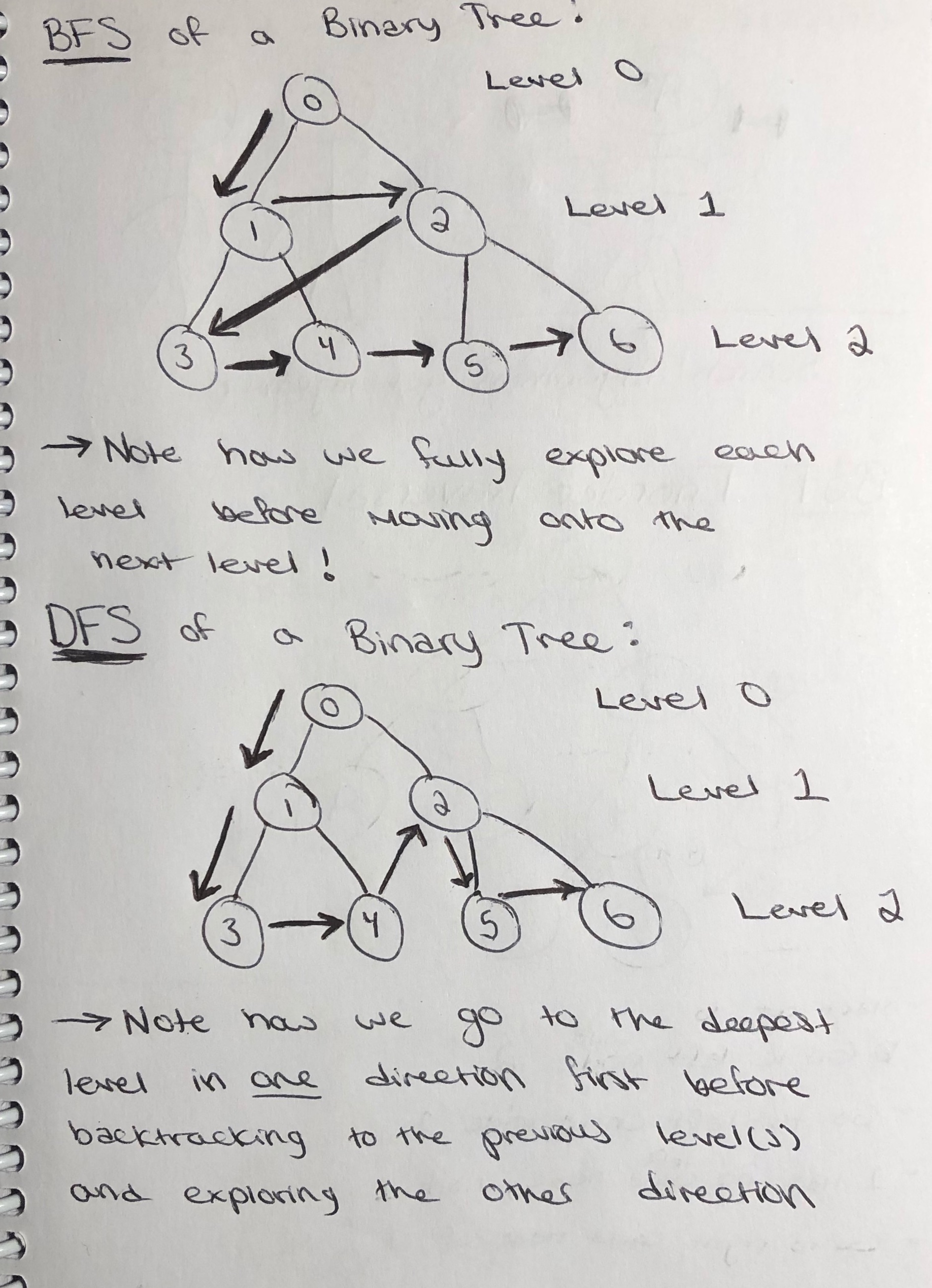
Depth-first search (DFS) is a common algorithm for traversing or searching tree or graph data structures. The DFS method is a search that goes as deeply as it can before backtracking to its last decision point if it reaches a dead end. An algorithm for DFS is sketched out below:
DFS(start, goal):
    n = start; the starting node
    S = a Stack

    S.push(n)  # Pushes starting node onto the stack
    while S is not empty:
        n = S.pop()  # Pops the newest node on the stack
        if n == goal:  # exit condition
            return n
        for all nodes w in get_neighbors(n):  # Explore neighbor locations
            if w has not been searched yet:
                label w as searched
                S.push(w)
The key part of this algorithm to note is the use of the stack. We know the stack is FIFO, so instead of exploring all the adjacent nodes first, we keep exploring in one direction until we can go no further (i.e. until something has blocked our path, or we have reached the end goal). This is where the algorithm gets its name -- we go as deep as we can to start. The time complexity for DFS is O$(n)$, since in the worst case we have to explore all $n$ vertices of the graph. Unlike the BFS and A* search algorithms, DFS is not guaranteed to find the shortest path.
Breadth-first search (BFS) is another common algorithm for searching a tree or graph data structures for a node or vertex that satisfies a given property. Unlike DFS, the BFS algorithm explores all nodes at the present "depth" prior to moving to the nodes at the next depth level. Because of this, BFS is guaranteed to find us the shortest path so long as the edges between nodes and vertices are not weighted. An algorithm for BFS is sketched out below:
BFS(start, goal):
    n = start; the starting node
    Q = a Queue

    Q.push(n)  # Pushes starting node onto the queue
    while Q is not empty:
        n = Q.pop()  # Pops the oldest node on the queue
        if n == goal:  # exit condition
            return n
        for all nodes w in get_neighbors(n):  # Explore neighbor locations
            if w has not been searched yet:
                label w as searched
                Q.push(w)
The key part of this algorithm to note is the use of the queue. We know the stack is LIFO, so all the adjacent nodes, which are pushed onto the queue first, are explored first before any nodes at the next depth level are. If you look closely at both pseudocode examples, there is essentially no difference besides the stack vs. queue aspect, which goes to show how we can get very different methods and outcomes from a small tweak to the underlying data structure used. Because of this minor difference, BFS will always find the shortest path where one exists, whereas DFS is not guaranteed to find the shortest path (it rarely does). The time complexity for BFS is also O$(n)$, since in the worst case we have to explore all $n$ nodes of the graph.
A* search is yet another graph traversal and path search algorithm. It is a "best-first" search algorithm that requires a weighted graph (cost to move between nodes can be measured in distance, time, etc.) in which we find the path on the graph with the smallest cost. To do this, A* maintains a tree of paths originating at the start node and extends those paths one step at a time until the goal is reached. In order to implement this, some auxiliary cost functions are required:
What A* does is select the path that minimizes $f(n)$. The algorithm terminates when path to extend is a completed path from start to goal; or there is no eligible path to extend. An algorithm for A* is sketched out below:
a_star(start, goal):
    n = start; the starting node
    to_explore = a Priority Queue
    explored = a dictionary

    g(n) = 0
    h(n) = manhattan distance from n to goal
    f(n) = g(n) + h(n)

    to_explore.insert(f(n), Node(n, n's parent, g(n), h(n)))
    explored[n] = g(n)

    while to_explore is not empty:
        e = to_explore.remove_min()
        n = e.item
        if n == goal:
            return n
        g(n) = n.cost

        for m in get_neighbors(n):
            g(m) = g(n) + 1  # cost is one step away from n
            if m not in explored or g(m) < explored[m]:  # second conditions says even if we have explored m,
            # we want to see if coming at it from n makes g(m) (and hence f(m)) smaller or not
                explored[m] = g(m)  # set the new/improved cost from start
                h(m) = Manhattan distance from m to goal  # set heuristic
                f(m) = g(m) + h(m)
                to_explore.insert(f(m), Node(m, m's parent, g(m), h(m))
The key part of this algorithm to note is the use of the priority queue. The priority queue enables us to remove the node having the smallest $f(n)$ value when determining which node to search next. Additionally, the reason we use a dictionary in the pseudocode above is that it allows us to easily update the cost to a node if it improves on a different path (i.e. if there is a better path going through another node). Also, note that the Manhattan distance between two points is simply the sum the absolute differences of their Cartesian coordinates. While BFS and A* can both find the shortest path in terms of actions (i.e. least number of vertices), only A* will find the least-cost path when the edges between vertices/nodes might be weighted. Once more, the time complexity for A* is O$(V + E)$, since in the worst case we have to explore all $V$ vertices and $E$ edges of the graph.
During this semester, we implemented all of DFS, BFS, and A* to solve rectangular mazes. The code is shown below:
class Contents(str, Enum):
    ''' create an enumeration to define what the visual contents of a Cell are;
        using str as a "mixin" forces all the entries to be strings; using an
        enum means no cell entry can be anything other than the options here
    '''
    EMPTY   = " "
    START   = "⦿" #"S"
    GOAL    = "◆" #"G"
    BLOCKED = "░" #"X"
    PATH    = "*" #"*"


class Position(NamedTuple):
    row: int
    col: int


class Cell:
    ''' allows us to use Cell as a data type -- an ordered triple of
        row, column, cell contents '''
    def __init__(self, row: int, col: int, contents: Contents):
        self._position = Position(row, col)
        self._contents = contents

    def get_position(self) -> Position:
        return Position(self._position.row, self._position.col)

    def mark_on_path(self) -> None:
        self._contents = Contents.PATH

    def is_blocked(self) -> bool:
        return self._contents == Contents.BLOCKED

    def is_goal(self) -> bool:
        return self._contents == Contents.GOAL

    def __str__(self) -> str:
        contents = "[EMPTY]" if self._contents == Contents.EMPTY else self._contents
        return f"({self._position.row}, {self._position.col}): {contents}"

    def __eq__(self, other) -> bool:
        return self._position.row == other._position.row and \
               self._position.col == other._position.col and \
               self._contents == other._contents


class Node:
    def __init__(self, cell: Cell, parent: Optional['Node'], cost: float = 0., heuristic: float = 0.):
        self.cell      = cell
        self.parent    = parent
        self.cost      = cost
        self.heuristic = heuristic

    def __str__(self):
        parent = "None" if self.parent is None else self.parent.cell
        return f"{self.cell} : parent = {parent}"

    def __lt__(self, other: 'Node'):
        f_of_n = self.cost + self.heuristic
        f_of_m = other.cost + other.heuristic
        return f_of_n < f_of_m


def manhattan(from_: Cell, to_: Cell) -> float:
    col_dist = abs(to_.get_position().col - from_.get_position().col)
    row_dist = abs(to_.get_position().row - from_.get_position().row)
    return col_dist + row_dist


class Maze:
    ''' class representing a 2D maxe of Cell objects '''

    ss_counter: int = 0  # states searched counter

    def __init__(self, rows: int = 10, cols: int = 10, prop_blocked: float = 0.2, \
                       start: Position = Position(0, 0), \
                       goal:  Position = Position(9, 9) ):
        '''
        Args:
            rows:          number of rows in the grid
            cols:          number of columns in the grid
            prop_blocked:  proportion of cells to be blocked
            start:         tuple indicating the (row,col) of the start cell
            goal:          tuple indicating the (row,col) of the goal cell
        '''
        self._num_rows = rows
        self._num_cols = cols
        self._start    = Cell(start.row, start.col, Contents.START)
        self._goal     = Cell(goal.row,  goal.col,  Contents.GOAL)

        # create a rows x cols 2D list of Cell objects, initially all empty
        self._grid: List[List[Cell]] = \
            [ [Cell(r,c, Contents.EMPTY) for c in range(cols)] for r in range(rows) ]

        # set the start and goal cells
        self._grid[start.row][start.col] = self._start
        self._grid[goal.row][goal.col]   = self._goal

        # put blocks at random spots in the grid, using given proportion;
        # start by creating a collapsed 1D version of the grid, then
        #   remove the start and goal, and then randomly pick cells to block;
        # note that we are using identical object references in both
        #   options and self._grid so that updates to options will be seen
        #   in self._grid (i.e., options is not a deep copy of cells)
        options = [cell for row in self._grid for cell in row]
        options.remove(self._start)
        options.remove(self._goal)
        blocked = random.sample(options, k = round((rows * cols - 2) * prop_blocked))
        for b in blocked: b._contents = Contents.BLOCKED
        '''
        # for example from slides
        pos = [(1,0),(1,3),(2,1),(2,4),(3,2),(5,1),(5,3),(5,4)]
        for p in pos:
            self._grid[p[0]][p[1]]._contents = Contents.BLOCKED
        '''

    def __str__(self) -> str:
        ''' returns a str version of the maze, showing contents, with cells
            deliminted by vertical pipes '''
        maze_str = ""
        for row in self._grid:  # row : List[Cell]
            maze_str += "|" + "|".join([cell._contents for cell in row]) + "|\n"
        return maze_str[:-1]  # remove the final \n

    def get_start(self): return self._start
    def get_goal(self):  return self._goal

    def get_search_locations(self, cell: Cell) -> List[Cell]:
        ''' return a list of Cell objects of valid places to explore
        Args:
            cell: the current cell being explored
        Returns:
            a list of valid Cell objects for further exploration
        '''
        # on_board() is a helper function that checks to make sure a given row (r) and column (c) index is inside
        # the maze board. We do not want to generate "possible" moves that are not on the board!
        def on_board(r, c):
            return r in range(len(self._grid)) and c in range(len(self._grid[0]))

        # The 'cell' parameter passed into this method is the current cell we are at on the board. We want to generate
        # the possible moves from this cell. To make things easier, we redefine the position of the cell on the
        # board using simple 'row' and 'col' variable names
        row = cell.get_position()[0]
        col = cell.get_position()[1]

        # The possible moves are North [-1, 0], West [0, -1], East [0, 1], South [1, 0]. The ordering I have placed
        # the possible moves in biases our search towards the southeast. Why? The reason is that we first push North,
        # then West, then East, then South. This means South will be pushed off the stack first, the East, etc. etc.,
        # which moves us in the southeast direction primarily. This makes sense when the start is in the
        # upper left of the board and the goal is in the bottom right. If the locations of the start and goal were
        # different we might want to change the ordering.

        # possible_moves = [[-1, 0], [0, -1], [0, 1], [1, 0]]

        # I changed the ordering to match what was in the slides -- now the bias is towards the east.
        possible_moves = [[-1, 0], [1, 0], [0, -1], [0, 1]]
        locations = []

        # We test if the new cell we generated from a move is valid using the on_board() function. If TRUE is returned,
        # the location is appended to a list of valid cells we can move to from the input cell. Again, it is important
        # to note that the ordering in which the locations are appended does matter! The locations North and West are
        # appended first so in our dfs() method they will be pushed to the bottom of the stack first and searched last,
        # biasing our search towards the SouthEast.
        for move in possible_moves:
            new_row = row + move[0]
            new_col = col + move[1]
            # print("row : " + str(new_row))
            # print("col : " + str(new_col))
            if on_board(new_row, new_col):
                if not self._grid[new_row][new_col].is_blocked():
                    locations.append(self._grid[new_row][new_col])
                else:
                    continue
            else:
                continue

        return locations

    def dfs(self) -> Optional[Node]:
        '''
        Use DFS + stack:
            stack: push new cells to be explored
            list:  cells already explored
        Return:
            current node if it is the goal
            None, if no goal can be found
        '''
        # First we create an empty stack and list. We will push nodes to be explored onto the stack and cells that
        # we have already explored into the explored list.
        stack = Stack()
        explored = []

        # We start by initializing the current_node as the start node, which has no parent node, and push it onto
        # the stack. We also add the start cell to the explored list so we don't go back to it at any point.
        current_node = Node(self.get_start(), None)
        stack.push(current_node)
        explored.append(current_node.cell)

        # As long as the stack is not empty and we have not reached the goal, there are still more locations to
        # search, so we keep looping. If the stack is empty before reaching the goal, there is no possible path
        # to the goal (due to "BLOCKED" cells)
        while not stack.is_empty() and current_node.cell != self.get_goal():
            current_node = stack.pop()

            self.ss_counter += 1

            # We check the possible search locations of the cell of the current_node we just popped from the top
            # of the stack. Before we push any of these locations onto the stack, we check to make sure the location
            # is not some cell we have already explored. If it is not, then we push that cell onto the stack as a node.
            # Its parent node is the current node. We also add all of those cells to the explored list. This is
            # because we don't want any other cells claiming to be the parent of these cells.

            if current_node.cell == self.get_goal():
                return current_node

            for cell in self.get_search_locations(current_node.cell):
                if cell not in explored:
                    # print("potential cell" + str(cell))
                    stack.push(Node(cell, current_node))
                    explored.append(cell)
                else:
                    continue
            # print(current_node)

        # Once we have exited the while loop, we have either reached the goal or run out of options. If the former,
        # we return the current_node, which should be the goal node. This node contains all the necessary information
        # about its path (this is in the loop). If we ran out of options and we couldn't reach the goal node,
        # we simply return None.

        return None

    def bfs(self) -> Optional[Node]:
        '''
        Use BFS + queue:
            queue: push new cells to be explored
            list:  cells already explored
        Return:
            current node if it is the goal
            None, if no goal can be found
        '''
        # First we create an empty queue and list. We will push nodes to be explored onto the queue and cells that
        # we have already explored into the explored list.
        queue = Queue()
        explored = []

        current_node = Node(self.get_start(), None)
        queue.push(current_node)
        explored.append(current_node.cell)

        # As long as the queue is not empty and we have not reached the goal, there are still more locations to
        # search, so we keep looping. If the queue is empty before reaching the goal, there is no possible path
        # to the goal (due to "BLOCKED" cells)
        while not queue.is_empty() and current_node.cell != self.get_goal():
            current_node = queue.pop()

            self.ss_counter += 1

            # print(current_node.cell)
            # We check the possible search locations of the cell of the current_node we just popped from the left
            # of the queue. Before we push any of these locations onto the queue, we check to make sure the location
            # is not some cell we have already explored. If it is not, then we push that cell onto the queue as a node.
            # Its parent node is the current node. We also add all of those cells to the explored list. This is
            # because we don't want any other cells claiming to be the parent of these cells.

            if current_node.cell == self.get_goal():
                return current_node

            for cell in self.get_search_locations(current_node.cell):
                if cell not in explored:
                    # print("potential cell" + str(cell))
                    queue.push(Node(cell, current_node))
                    explored.append(cell)
                else:
                    continue
            # print(current_node)

        # Once we have exited the while loop, we have either reached the goal or run out of options. If the former,
        # we return the current_node, which should be the goal node. This node contains all the necessary information
        # about its path (this is in the loop). If we ran out of options and we couldn't reach the goal node,
        # we simply return None.

        return None

    def a_star(self) -> Optional[Node]:
        ''' method to implement the A* algorithm for searching a maze
        Returns:
            the goal Node, if a path is found, or None if no path from start
            to goal
        '''

        to_explore = PriorityQueue()   # to keep track of locations to explore
        explored   = dict()  # to associate location:cost, perhaps for later updating

        # start by handling the start node
        n = self._start
        g_n = 0.0  # costs zero to get from start to start
        h_n = manhattan(self._start, self._goal)
        f_n = g_n + h_n

        # add the start node to the PQ of locations to be explored;
        # f(n) is the priority for the PQ; note that only the start node has
        # None for the parent
        to_explore.insert(f_n, Node(n, None, g_n, h_n))
        explored[n.get_position()] = g_n  # use position for the dict key

        while not to_explore.is_empty():
            entry = to_explore.remove_min()
            current_node = entry._value

            self.ss_counter += 1

            if current_node.cell == self.get_goal():
                return current_node

            for m in self.get_search_locations(current_node.cell):
                g_m = current_node.cost + 1  # cost is one step away from current_node
                # check if position has been explored. If it has we skip over unless the cost from the current_node
                # is less than through the node we previously explored it from.
                if (m.get_position() not in explored) or (g_m < explored[m.get_position()]):
                    explored[m.get_position()] = g_m  # set the new/improved cost from start
                    h_m = manhattan(m, self.get_goal())  # set heuristic
                    f_m = g_m + h_m
                    to_explore.insert(f_m, Node(m, current_node, g_m, h_m))
                else:
                    continue

        # Once we have exited the while loop, we have either reached the goal or run out of options. If the former,
        # we return the current_node, which should be the goal node. This node contains all the necessary information
        # about its path (this is in the loop). If we ran out of options and we couldn't reach the goal node,
        # we simply return None.

        return None

    def show_path(self, node: Node) -> None:
        '''
        Args :
            The output from dfs() (a Node object) should be
            passed into this method. This means the Node passed in
            will either be the start node or goal node.
        Returns :
            None -- The goal of this method is simply to
            display the maze with the path (or lack thereof).
        '''
        path = []
        # If the node passed as the parameter is the goal node then we will be able to trace all the parent nodes
        # back to the start. We add the cell of each corresponding node we trace back through to a list. This list is
        # the path from the goal node to the start node. If the start node is passed, the parent will be None and
        # the loop is skipped. In this case the function will just print a blank maze (same as calling print() on
        # a Maze() object)
        while node.parent is not None:
            path.append(node.cell)
            # print(node.cell)
            node = node.parent
        path.append(node.cell)

        # The path is from the goal node to the start node so we need to reverse the path.
        path.reverse()

        # We change the symbol of each cell on the path to "PATH" so when we print the Maze object it will display
        # the path.
        for cell in path:
            if cell != self._start and cell != self._goal:
                cell.mark_on_path()
        print(self)

        return None

    def get_path(self, node: Node) -> list:
        '''
        Args :
            The output from dfs(), bfs(), or a_star() (a Node object)
            should be passed into this method. This means the Node passed
            in will either be the start node or goal node.
        Returns :
            The path as a list of positions (tuple).
        '''
        path = []

        while node.parent is not None:
            path.append(node.cell.get_position())
            # print(node.cell)
            node = node.parent
        path.append(node.cell.get_position())

        # The path is from the goal node to the start node so we need to reverse the path.
        path.reverse()

        return path
The implementations of Stack, Queue, and PriorityQueue can be found in the respective
documents for those data structures.
When comparing searching algorithms such as DFS and BFS, one might be curious as to when it is ideal to use one or the other. As the cited article on applications of searching algorithms in AI (artificial intelligence) notes, BFS (and A*) can be used when you want to find the shortest path. However, DFS often requires less memory and can take less time when the solution is farther away (despite similar worst-case time complexity, there can still be sizable differences in best-case and average-case!).